
Disclaimer: This blog post is based on the paper 'Validation of the Vertical Corrector Magnets for HESR Using COMSOL Modelling and Python Data Analysis' presented at ATEE 2025 – The 14th International Symposium on Advanced Topics in Electrical Engineering, October 9-11, 2025, Bucharest, Romania (https://atee.upb.ro/atee2025/) . The full paper is available on IEEE Xplore at: https://ieeexplore.ieee.org/document/11299947
Introduction
In the realm of particle accelerators, precision in electromagnetic design is paramount. The High-Energy Storage Ring (HESR) at the Facility for Antiproton and Ion Research (FAIR) (https://en.wikipedia.org/wiki/Facility_for_Antiproton_and_Ion_Research) in Germany represents a cutting-edge project where normal-conducting magnets play a critical role in steering and correcting charged particle beams. As part of Romania's in-kind contribution to FAIR, the National Institute for R&D in Electrical Engineering ICPE-CA (https://www.icpe-ca.ro/) manufactured a series of vertical corrector magnets. This blog explores the validation process for these magnets, emphasizing the electromagnetics principles involved and the pivotal role of Python in data analysis, complemented by COMSOL Multiphysics simulations.
The Electromagnetic Backbone of Particle Accelerators
Particle accelerators rely on electromagnetic fields to guide beams of charged particles at relativistic speeds. Electromagnets function akin to optical lenses: dipoles deflect trajectories, quadrupoles focus beams, and higher-order magnets like hexapoles correct aberrations. In HESR, vertical corrector magnets—essentially dipole electromagnets—provide fine adjustments to the beam path, compensating for misalignments or external perturbations.
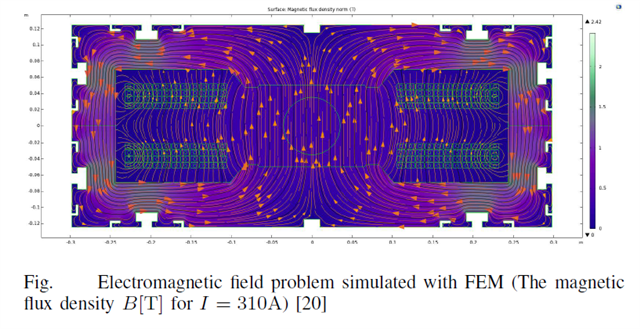
These magnets feature an E-shaped yoke made from laminated soft iron with nonlinear B-H characteristics, wound with copper coils (44 turns each) carrying DC currents up to 310 A. The design targets a central magnetic flux density of 0.333 T in a 0.100 m aperture, with field measurements extending to a 0.036 m radius. Key challenges in electromagnetics include achieving uniform field distribution, minimizing hysteresis, and accounting for saturation effects in the ferromagnetic core.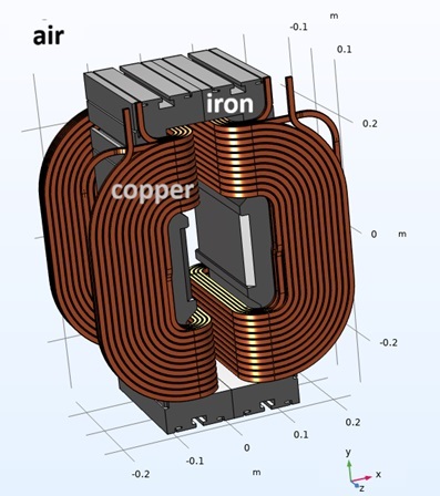
To validate series production, we focused on four core magnetic characteristics:
- Local excitation curve (f1): Central flux density per unit current.
- Integral excitation curve (f2): Integrated field along the longitudinal axis per unit current.
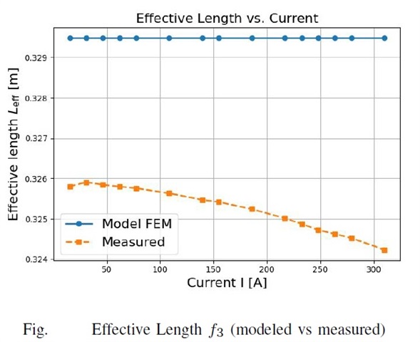
- Effective magnetic length (f3 ): Normalized longitudinal field extension.
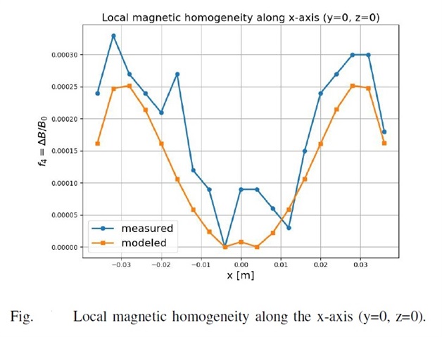
- Local homogeneity curve (f4): Relative field variation across the transverse axis.
These metrics ensure the magnets meet stringent tolerances for beam stability, where even minor deviations can lead to beam loss or reduced luminosity.
Numerical Modeling with COMSOL: Capturing Electromagnetic Behavior
COMSOL Multiphysics served as the simulation backbone, solving magnetostatic problems governed by Maxwell's equations:
∇⋅B=0,∇×H=J,B=μH
We modeled the magnet in both 2D and 3D, exploiting symmetry to reduce computational domains (e.g., quarter-section in 2D, eighth in 3D). The 2D model, with a mesh of ~268,000 triangular elements, was ideal for quick iterations on local properties like f1 and f4. For integral quantities (f2, f3), 3D models (~75,000 tetrahedral elements) captured end effects and fringe fields, using the magnetic vector potential formulation:
∇×(ν∇×A)=J
Boundary conditions included magnetic insulation on outer surfaces and symmetry constraints (Dirichlet on one axis, Neumann on another). Nonlinear material properties were incorporated via the B-H curve, and current densities were defined subdomain-wise (e.g., helical approximations in coils).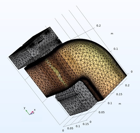
Simulations ran for excitation currents from ±15.5 A to ±310 A, revealing field distributions with peak densities near poles and uniformity in the good-field region. For instance, at 310 A, the central B-field matched measurements within 0.1%, highlighting COMSOL's accuracy in predicting saturation and flux leakage.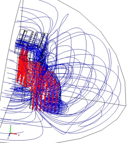
Python's Role in Electrical Engineering: Data Processing and Validation
While COMSOL handles the physics, Python bridges the gap between raw measurements and insightful analysis. Using libraries like NumPy, Pandas, SciPy, and Matplotlib, we processed Hall probe data from the measurement campaign. Python's strength in electrical engineering lies in its ability to handle large datasets, perform statistical analyses, and visualize complex electromagnetic behaviors efficiently.
Local Excitation Curve Processing Script loads currents I and central fields B₀, computes normalized f₁ = B₀/I, and plots:
- B₀ vs I (linear-ish with saturation at high |I|)
- B₀/I vs I (shows permeability drop due to saturation)
Code example (simplified):
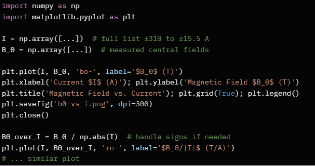
This revealed hysteresis minimal and saturation onset, with f₁ stable ~0.00109 T/A at low currents.
Integral Excitation Curve For longitudinal profiles, scripts plot B_x(z) for selected currents (symmetric positive/negative), then compute integrated BL/I separately for positive/negative ramps to check consistency.
- Multi-line plot: B_x vs z for I = ±62, ±186, ±310 A shows good symmetry and end roll-off.
- BL/I vs I plots: very flat (~0.000333–0.000335 Tm/A), confirming effective length near-constant.
Code snippet for multi-current plot:
Local Homogeneity Analysis Most advanced scripts compare transverse profiles (y-axis, -0.036 to +0.036 m):
- Interpolate central B₀_model and B₀_meas.
- Compute ΔB/B₀ for both.
- Relative error: (measured - model)/model * 100%, with stats (mean, max, min printed).
- Plots: ΔB/B₀ overlaid, error % curve, with ±0.01% limits and markers for exceedances.
- Additional: loadtxt from .txt files for normalized deviations at specific positions (ex. 33 mm variants).
Example stats output: mean relative error ~0.4–0.6%, max <1%, confirming uniformity within tolerances in central region.
These scripts enabled rapid iteration: load data, compute metrics, visualize deviations, flag outliers – critical for series validation magnets.
Key Insights from Python Analysis
- Local Excitation: Mean relative error of 0.62% across currents, with Python revealing minimal hysteresis (differences <0.1% between positive/negative ramps).
- Integral Excitation: Errors <1.5%, but Python highlighted larger discrepancies (~11%) at magnet ends, attributable to fringe effects—prompting model refinements.
- Effective Length: Python fitted empirical models (Leff=lFE+2hk L_{eff} = l_{FE} + 2hk ), yielding k≈0.38-0.40, aligning simulations and measurements within 1.3%.
- Homogeneity: Field uniformity within ±0.5% in the good region; Python's error plots showed peaks at low ΔB points, but overall agreement confirmed design tolerances.
Python's integration with COMSOL (via LiveLink or data export) enabled hybrid workflows: simulate in COMSOL, analyze in Python, iterate designs.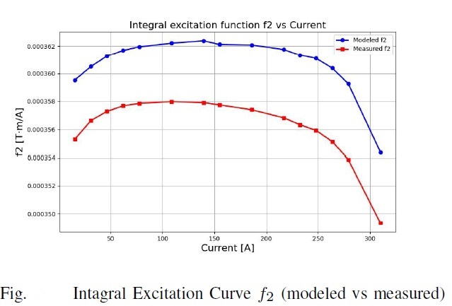
Practical Implications for Electromagnetics in Industry
In electrical engineering, this validation underscores Python's versatility beyond scripting—it's a tool for real-time diagnostics in magnet production.
Electromagnetically, the study validates normal-conducting designs for high-energy applications. Challenges like core saturation (evident in nonlinear B-H) were mitigated through precise modeling, ensuring HESR's beam correction meets FAIR's specs.
Comparisons showed 2D models suffice for transverse properties, while 3D is essential for longitudinal integrals—guiding efficient simulation strategies.
Conclusions and Future Directions
The synergy of COMSOL modeling and Python analysis validated the HESR vertical correctors with high fidelity. This workflow not only confirms manufacturing quality but exemplifies how electromagnetics principles, powered by computational tools, advance accelerator technology.
